GATE ECE 2013 | GATE ECE Year Wise Previous Years Questions

GATE ECE 2013

MCQ (Single Correct Answer)

-0.6

The signal flow graph for a system is given below. The transfer function $$\frac{Y(s)}{U(s)}$$ for this system is GATE ECE 2013 Control Systems - Signal Flow Graph and Block Diagram Question 18 English

GATE ECE 2013 Control Systems - Signal Flow Graph and Block Diagram Question 18 English

$$\frac{s+1}{5s^2+6s+2}$$

$$\frac{s+1}{s^2+6s+2}$$

$$\frac{s+1}{s^2+4s+2}$$

$$\frac{1}{5s^2+6s+2}$$

GATE ECE 2013

MCQ (Single Correct Answer)

-0.3

The Bode plot of a transfer function G (s) is shown in the figure below. GATE ECE 2013 Control Systems - Frequency Response Analysis Question 56 English

GATE ECE 2013 Control Systems - Frequency Response Analysis Question 56 English

The gain (20 log $$\left| {G(s)} \right|$$ ) is 32 dB and -8dB at 1rad/s and 10rad/s respectively. The phase is negative for all $$\omega .$$ Then G(s) is

$${\textstyle{{39.8} \over s}}$$

$${\textstyle{{39.8} \over {{s^2}}}}$$

$${\textstyle{{32} \over {{s}}}}$$

$${\textstyle{{32} \over {{s^2}}}}$$

GATE ECE 2013

MCQ (Single Correct Answer)

-0.6

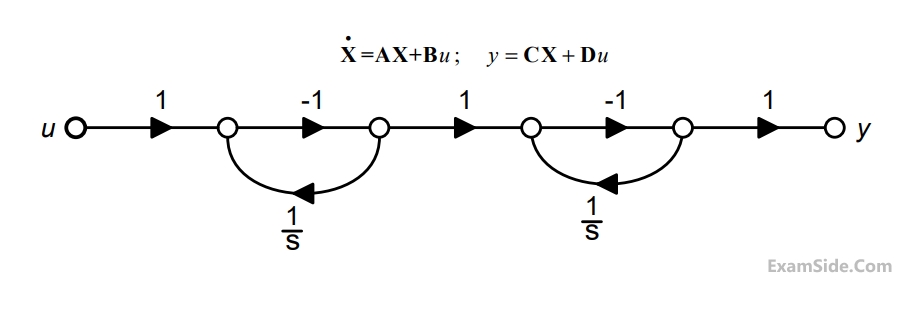
The state diagram of a system is shown below. A system is shown below. A system is described by the state variable equations GATE ECE 2013 Control Systems - State Space Analysis Question 23 English

GATE ECE 2013 Control Systems - State Space Analysis Question 23 English

The state transition matrix e^At of the system shown in the figure above is

$$\left[ {\matrix{ {{e^{ - t}}} & 0 \cr {t{e^{ - t}}} & {{e^{ - t}}} \cr } } \right]$$ v

$$\left[ {\matrix{ {{e^{ - t}}} & 0 \cr { - t{e^{ - t}}} & {{e^{ - t}}} \cr } } \right]$$

$$\left[ {\matrix{ {{e^{ - t}}} & 0 \cr {{e^{ - t}}} & {{e^{ - t}}} \cr } } \right]$$

$$\left[ {\matrix{ {{e^{ - t}}} & { - t{e^{ - t}}} \cr 0 & {{e^{ - t}}} \cr } } \right]$$

GATE ECE 2013

MCQ (Single Correct Answer)

-0.6

The state diagram of a system is shown below. A system is shown below. A system is described by the state variable equations GATE ECE 2013 Control Systems - State Space Analysis Question 24 English

GATE ECE 2013 Control Systems - State Space Analysis Question 24 English

The state-variable equations of the system shown in the figure above are

$$\eqalign{ & \mathop X\limits^ \bullet = \left[ {\matrix{ { - 1} & 0 \cr 1 & { - 1} \cr } } \right]X + \left[ {\matrix{ { - 1} \cr 1 \cr } } \right]u \cr & y = \left[ {\matrix{ 1 & { - 1} \cr } } \right]X + u \cr} $$

$$\eqalign{ & \mathop X\limits^ \bullet = \left[ {\matrix{ { - 1} & 0 \cr { - 1} & { - 1} \cr } } \right]X + \left[ {\matrix{ { - 1} \cr 1 \cr } } \right]u \cr & y = \left[ {\matrix{ { - 1} & { - 1} \cr } } \right]X + u \cr} $$

$$\eqalign{ & \mathop X\limits^ \bullet = \left[ {\matrix{ { - 1} & { - 1} \cr 0 & { - 1} \cr } } \right]X + \left[ {\matrix{ { - 1} \cr 1 \cr } } \right]u \cr & y = \left[ {\matrix{ 1 & { - 1} \cr } } \right]X - u \cr} $$

PREVIOUS NEXT

GATE ECE Papers

All year-wise previous year question papers

2026