Frequency Response Analysis · Control Systems · GATE ECE
Marks 1
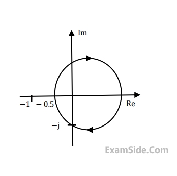
The Nyquist plot of a system is given in the figure below. Let $\omega_{\mathrm{P}}, \omega_Q, \omega_R$, and $\omega_{\mathrm{S}}$ be the positive frequencies at the points $P, Q, R$, and $S$, respectively. Which one of the following statements is TRUE?

In the context of Bode magnitude plots, 40 dB/decade is the same as ______.
The open loop transfer function of a unity negative feedback system is $$G(s) = {k \over {s(1 + s{T_1})(1 + s{T_2})}}$$, where $$k,T_1$$ and $$T_2$$ are positive constants. The phase cross-over frequency, in rad/s, is
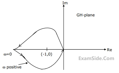
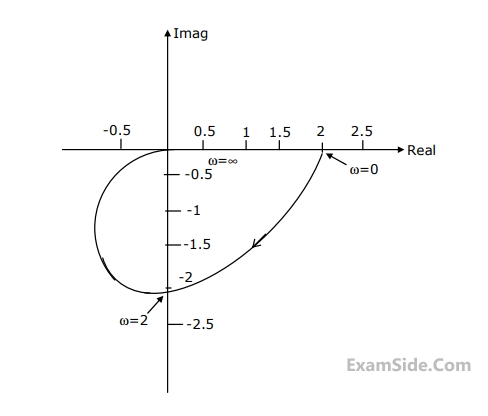
Consider a closed-loop control system with unity negative feedback and KG(s) in the forward path, where the gain K = 2. The complete Nyquist plot of the transfer function G(s) is shown in the figure. Note that the Nyquist contour has been chosen to have the clockwise sense. Assume G(s) has no poles on the closed right-half of the complex plane. The number of poles of the closed-loop transfer function in the closed right-half of the complex plane is ___________.


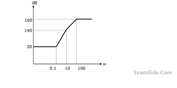
 The gain (20 log $$\left| {G(s)} \right|$$ ) is 32 dB and -8dB at 1rad/s and 10rad/s respectively. The phase is negative for all $$\omega .$$ Then G(s) is

Marks 2
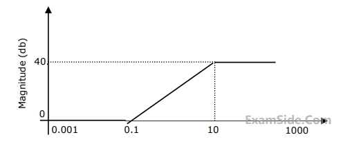
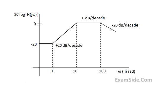
The asymptotic magnitude Bode plot of a minimum phase system is shown in the figure. The transfer function of the system is $$(s) = {{k{{(s + z)}^a}} \over {{s^b}{{(s + p)}^c}}}$$, where $$k,z,p,z,b$$ and $$c$$ are positive constants. The value of $$(a + b + c)$$ is ___________ (rounded off to the nearest integer)

A system with transfer function $G(s)=\frac{1}{(s+1)(s+a)}, a>0$ is subjected to input $5 \cos 3 t$. The steady state output of the system is $\frac{1}{\sqrt{10}} \cos (3 t-1.892)$. The value of $a$ is
$$G(s) = {{{n_0}} \over {{s^3} + {d_2}{s^2} + {d_1}s + {d_0}}}$$.

Consider the negative unity feedback configuration with gain k in the feedforward path. The closed loop is stable for k < k0. The maximum value of k0 is ______.
$$G(s) = {K \over {s\left( {s + 2} \right)}}$$
The peak resonant magnitude Mr of the closed-loop frequency response is 2. The corresponding value of the gain K (correct to two decimal places) is _________.

 If 0 < K < 1, then number of poles of the closed loop transfer function that lie in the right half of the s-plane is
 The value of p1 is ________
 The positive value of 𝑘 for which the gain margin of the loop is exactly 0 dB and the phase margin
of the loop is exactly zero degree is ____
The positive value of 𝑘 for which the gain margin of the loop is exactly 0 dB and the phase margin
of the loop is exactly zero degree is ____ The unit step response of the system approaches a steady state value of ______.

If the system is connected in a unity negative feedback configuration, the steady state error of the closed loop system, to a unit ramp input, is
 The signal flow graph that DOES NOT model the plant transfer function H(s) is
The gain margin of the system under closed loop unity negative feedback is
The signal flow graph that DOES NOT model the plant transfer function H(s) is
The gain margin of the system under closed loop unity negative feedback is
 The gain and phase margins of G(s) for closed loop stability are
Which of the foloowing statements is true?
The gain and phase margins of G(s) for closed loop stability are
Which of the foloowing statements is true?
The output of this system to the sinusoidal input x(t) = 2cos(t) for all time 't' is
The frequency response H(ω) of the system in terms of angular frequency 'ω' is given by h( ω)

With the value of "a" set for phase-margin of $$\pi $$/4, the value of unit-impulse response of the open-loop system at t = 1 second is equal to


The gain margin of the system is
Marks 5

Marks 8
Sketch Nyquist plot for the system and there from obtain the gain margin and the phase margin.
(a) Determine G(s), if it is known that the system is of minimum phase type.
(b) Estimate the phase at each of the corner frequencies.
